Diffusion and Ionic Transport

msd (`plt_msd.py`)

Plots mean square displacement (MSD) for all directions.

Input File: msd.out with time and MSD_x/y/z in its first four columns. This accepts the four-column output from gpumdkit.sh -calc msd and the first four columns of GPUMD compute_msd output.

The slope annotations use the middle 40%-80% of the MSD series.

bash

gpumdkit.sh -plt msd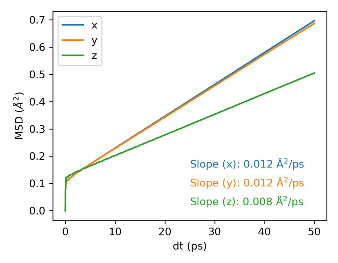

msd_all (`plt_msd_all.py`)

Plots MSD for all atomic species separately when using all_groups in GPUMD.

Input File: msd.out (computed with all_groups option)

Requirements: Must use all_groups in the compute_msd command in run.in. For multiple groups, GPUMD appends group data; inspect that layout rather than assuming the file has the seven columns of a single-group result.

bash

gpumdkit.sh -plt msd_all msd.out Li P S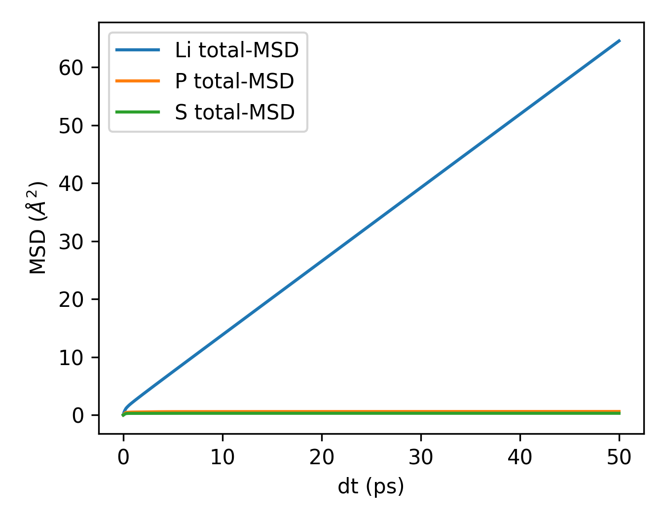

msd_conv (`plt_msd_convergence_check.py`)

Checks convergence of MSD calculations across different time windows.

Input File: msd_step*.out (computed with save_every option)

Requirements: Use save_every in the compute_msd command.

Purpose: Verify MSD has converged sufficiently for accurate diffusion coefficient calculation.

bash

gpumdkit.sh -plt msd_conv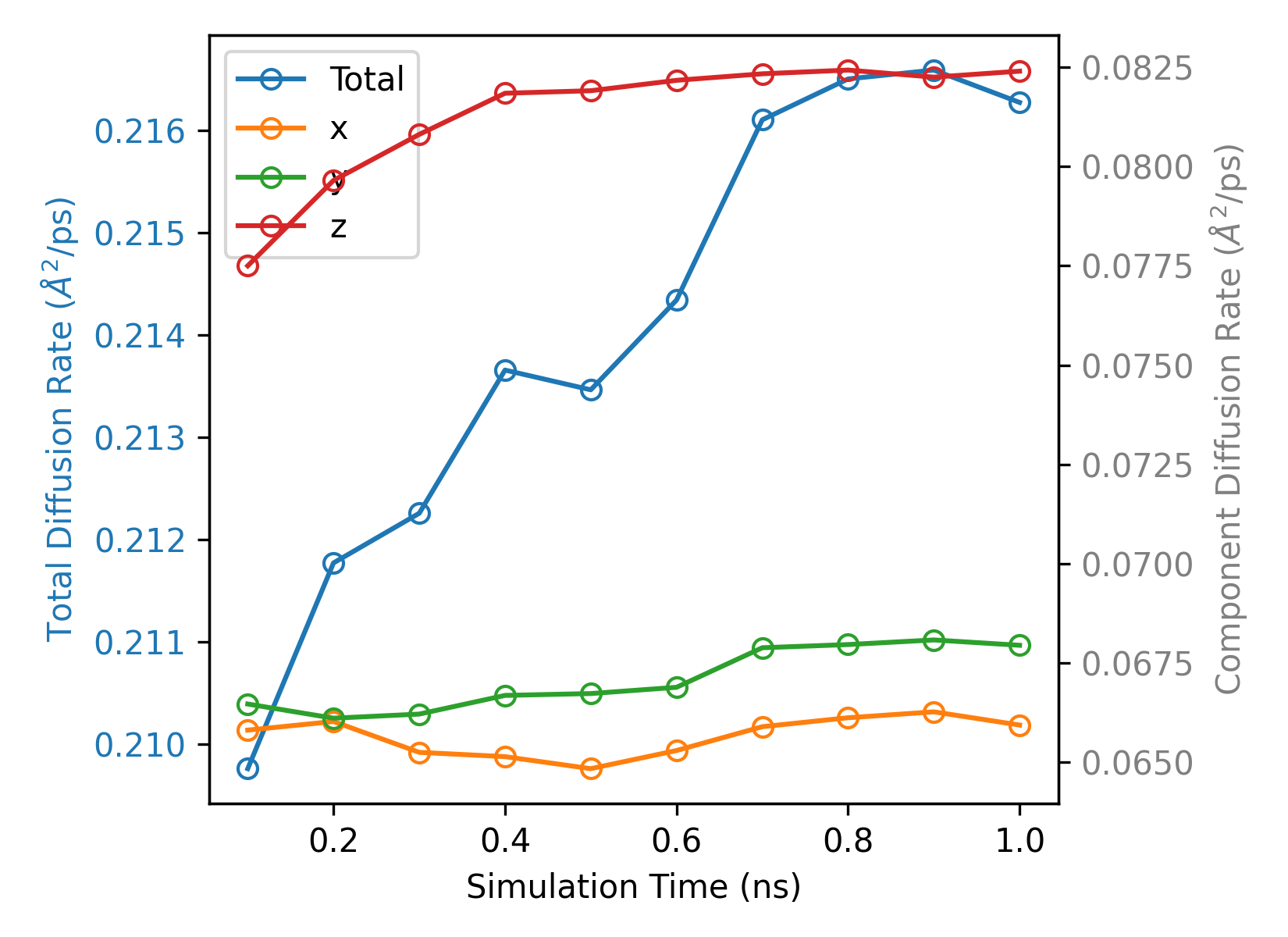

sdc (`plt_sdc.py`)

Plots self-diffusion coefficient (SDC) vs time.

Input File: a single-group seven-column msd.out from GPUMD compute_msd: time, MSD_x/y/z, and SDC_x/y/z. The four-column file from -calc msd is not sufficient for this plot.

bash

gpumdkit.sh -plt sdc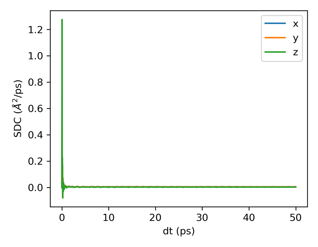

msd_sdc (`plt_msd_sdc.py`)

Plots MSD and self-diffusion coefficient (SDC) side by side. The slope annotations use the middle 40%-80% of the MSD series; the inset shows the last 80% of the SDC data with a moving-average overlay.

Input File: a single-group seven-column msd.out from GPUMD compute_msd: time, MSD_x/y/z, and SDC_x/y/z. The four-column file from -calc msd is not sufficient for this plot.

bash

gpumdkit.sh -plt msd_sdc

D (`plt_arrhenius_d.py`)

Creates Arrhenius plot for diffusivity (log10 D vs 1000/T).

Input Files: *K/msd.out files (each temperature subdirectory should contain an msd.out)

bash

gpumdkit.sh -plt arrhenius_d
gpumdkit.sh -plt D             # Alternative command

Activation-energy output format:

text

Activation Energy: <Ea> eV, R2 = <R2>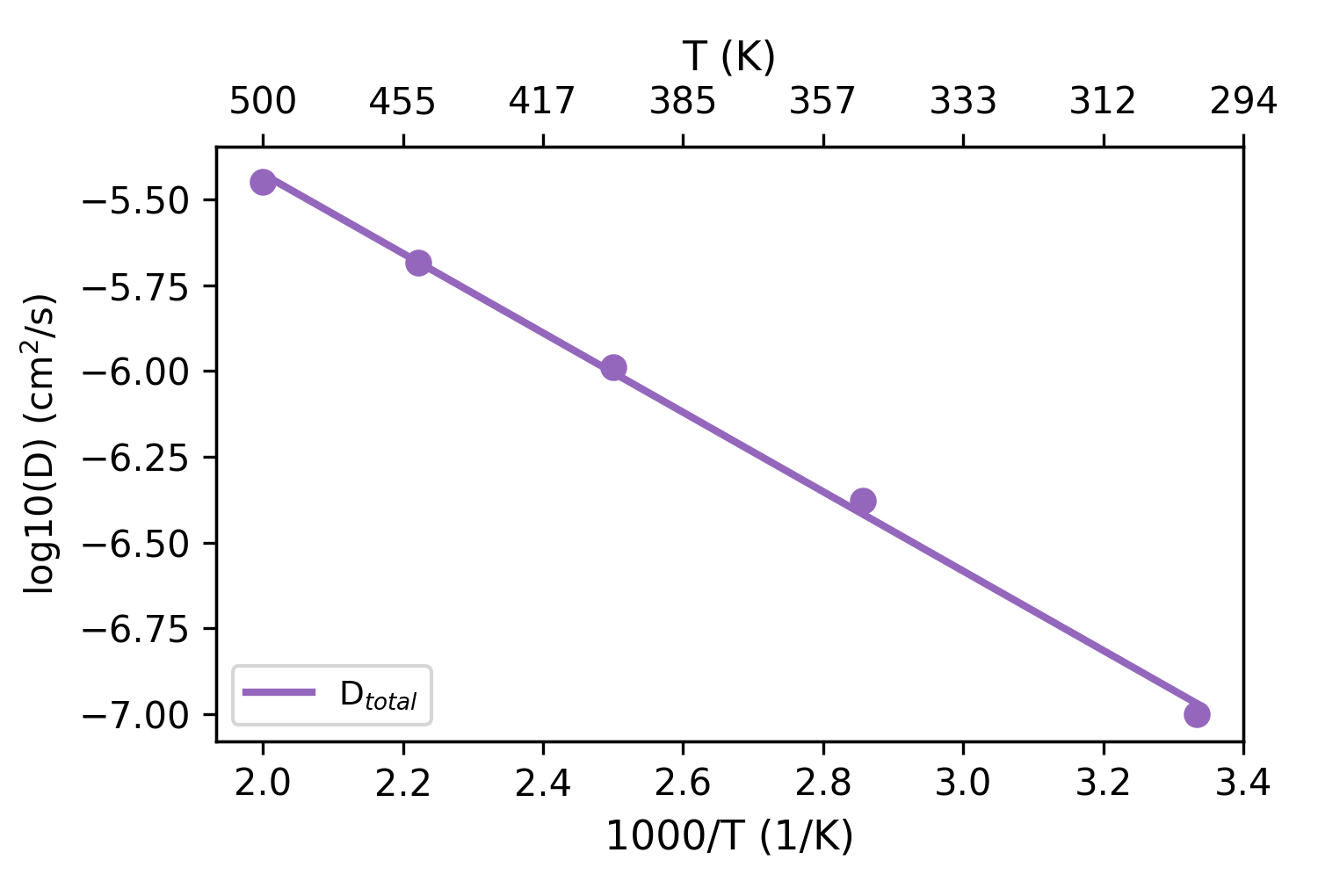

D_PT (`plt_arrhenius_d_PT.py`)

Creates a piecewise Arrhenius diffusivity plot around a user-specified phase-transition temperature. The transition-temperature point is included in both the LowT (T <= Tc) and HighT (T >= Tc) fits.

Input Files: *K/msd.out files

bash

gpumdkit.sh -plt D_PT 380
gpumdkit.sh -plt D_PT 380 save

The legend reports the activation energy of each branch as HighT (xx eV) and LowT (xx eV).

D_xyz (`plt_arrhenius_d_xyz.py`)

Calculates diffusion coefficients from msd.out in temperature folders for the x/y/z directions, generates a directional Arrhenius plot, and extracts the activation energy of each component.

Input Files: *K/msd.out files

bash

gpumdkit.sh -plt D_xyz

Assumptions of the conductivity plots (sigma, sigma_PT, sigma_xyz)

These conductivity plots use the first temperature's model.xyz to count Li and Na together, assume unit charge, and apply the same ion count and replication across temperatures. Use them for one mobile Li or Na species with matching MSD columns; other species, mixed carriers, or changing composition require a separate calculation. They fit the 40%–80% MSD interval and extrapolate conductivity to 300 K using the Nernst–Einstein relation. Validate the diffusive interval and the extrapolation range before interpreting the results.

sigma (`plt_arrhenius_sigma.py`)

Creates Arrhenius plot for ionic conductivity (log10(σ·T) vs 1000/T).

Input Files: thermo.out and msd.out in each *K/ directory; model.xyz and optional run.in in the first temperature directory

bash

gpumdkit.sh -plt arrhenius_sigma
gpumdkit.sh -plt sigma         # Alternative command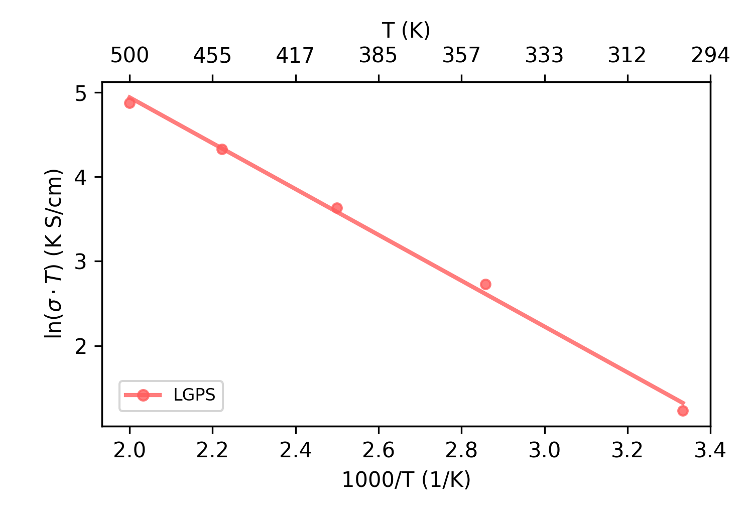

sigma_PT (`plt_arrhenius_sigma_PT.py`)

Creates a piecewise Arrhenius ionic-conductivity plot around a user-specified phase-transition temperature. The transition-temperature point is included in both the LowT (T <= Tc) and HighT (T >= Tc) fits. The 300 K conductivity is extrapolated from the branch on the same side of the transition as 300 K.

Input Files: thermo.out and msd.out in each *K/ directory; model.xyz and optional run.in in the first temperature directory

bash

gpumdkit.sh -plt sigma_PT 380
gpumdkit.sh -plt sigma_PT 380 save

The legend reports the activation energy of each branch as HighT (xx eV) and LowT (xx eV).

Phase-transition Arrhenius ionic conductivity

sigma_xyz (`plt_arrhenius_sigma_xyz.py`)

Calculates the ionic conductivity from MSD and thermo data in temperature folders for the x/y/z directions, plots the directional Arrhenius relationship, and extracts the activation energy of each direction using the Nernst-Einstein relation.

Input Files: thermo.out and msd.out in each *K/ directory; model.xyz in the first temperature directory

bash

gpumdkit.sh -plt sigma_xyz

PreviousMD and Structure NextHeat Transport and Phonons

Edit this page

Diffusion and Ionic Transport