🧲 Polar Material Analysis
This tutorial covers GPUMDkit calculator options 406-410 and the plane-grid plotting workflow.
Script Location: Scripts/calculators/ and Scripts/plt_scripts/
This tutorial includes both general and system-specific tools:
nlist,disp, andavg-structare broadly useful for structure/trajectory analysis.oct-tiltis for octahedral environments (requires 6 neighbors around each center).pol-abo3is specific toABO3polarization analysis.
Overview
| Step | CLI Command | Main Input | Output |
|---|---|---|---|
| Build neighbor list | gpumdkit.sh -calc nlist ... |
model.xyz |
nl-*.dat |
| Calculate displacement | gpumdkit.sh -calc disp ... |
trajectory + nl-*.dat |
displacements.dat |
| Average trajectory | gpumdkit.sh -calc avg-struct ... |
trajectory | averaged extxyz |
| Octahedral tilt | gpumdkit.sh -calc oct-tilt ... |
trajectory + B-O neighbor list | tilt-angle table |
| ABO3 polarization | gpumdkit.sh -calc pol-abo3 ... |
trajectory + neighbor lists | polarization table |
| Plane-grid plot | gpumdkit.sh -plt plane-grid ... |
structure + displacement data | plane profile plot |
Dependency
These scripts require ferrodispcalc:
Interactive mode entry
Options 406-410 are the core functions for this tutorial. The sections below explain when to use each one and how to run it.
The calculator menu is:
+----------------------------------------------------------+
|                     CALCULATOR TOOLS                     |
+----------------------------------------------------------+
| 401) Calc ionic conductivity                             |
| 402) Calc properties by nep                              |
| 403) Calc descriptors of specific elements               |
| 404) Calc density of atomistic states (DOAS)             |
| 405) Calc nudged elastic band (NEB) by nep               |
| 406) Build neighbor list                                 |
| 407) Calc displacement from trajectory                   |
| 408) Calc averaged structure                             |
| 409) Calc octahedral tilt                                |
| 410) Calc polarization for ABO3                          |
| 411) Minimize structure by nep                           |
| 412) Calc mean square displacement (MSD) from trajectory |
+----------------------------------------------------------+
| 000) Return to the main menu                             |
+----------------------------------------------------------+
Input the function number:
For full argument details, use:
gpumdkit.sh -calc nlist -h
gpumdkit.sh -calc disp -h
gpumdkit.sh -calc avg-struct -h
gpumdkit.sh -calc oct-tilt -h
gpumdkit.sh -calc pol-abo3 -h
gpumdkit.sh -plt plane-grid -h
406) Build neighbor list (calc_neighbor_list.py)
Build neighbor lists for selected center and neighbor elements.
When to use it:
This is usually the first step before disp, oct-tilt, and pol-abo3, because those scripts read nl-*.dat neighbor files.
Usage
# Example 1: Ti-O nearest 6 neighbors for octahedral analysis
gpumdkit.sh -calc nlist -i model.xyz -c 4.0 -n 6 -C Ti -E O -o nl-Ti-O.dat

# Example 2: Pb/Sr-O nearest 12 neighbors for A-site centered analysis
gpumdkit.sh -calc nlist -i model.xyz -c 4.0 -n 12 -C Pb Sr -E O
Arguments (complete)
-i, --input: Input structure file. Default:model.xyz.-x, --index: Frame index to read from input. Default:0.-c, --cutoff(required): Neighbor search cutoff (Angstrom).-n, --neighbor-num(required): Number of neighbors per center.-d, --defect: Defect mode. If enabled and neighbors are insufficient, missing slots are filled with the center index.-C, --center-elements(required): Center species list.-E, --neighbor-elements(required): Neighbor species list.-o, --output: Output file path. Default:nl-<center>-<neighbor>.dat.
Output file
- Main output: neighbor list text file (for example
nl-Ti-O.dat). - The file is a 2D integer array with shape
(n_center, neighbor_num + 1). Each row corresponds to one center atom: the first column is the center index, and the remaining columns are its neighbor indices (all 1-based).
407) Calc displacement from trajectory (calc_displacement.py)
Compute local displacement vectors from a trajectory/model and a neighbor list.
Usage
# Example 1: single-frame displacement from model.xyz
gpumdkit.sh -calc disp -i model.xyz -n nl-Ti-O.dat -o disp_model.dat

# Example 2: use the last 20% frames in movie.xyz
gpumdkit.sh -calc disp -i movie.xyz -n nl-Ti-O.dat -l 0.2 -o displacements.dat
Arguments (complete)
-i, --input: Input xyz file. Default:model.xyz.-n, --neighbor-list(required): Neighbor list file fromnlist.-o, --output: Output file. Default:displacements.dat.-s, --start: Slice start index. Default:0.-t, --stop: Slice stop index. Default: end.-p, --step: Slice step. Default:1.-l, --last: Select trailing frames. Integer: lastNframes.0 < value < 1: last ratio of frames.-l/--lastis mutually exclusive with-s/-t/-p.
Output file
- Main output:
displacements.dat(or your custom output name). - The saved text file is a 2D array: for a single-frame input, its shape is
(n_center, 3); for a multi-frame input, it is(n_selected_frame * n_center, 3)in frame-major order. The three columns aredx,dy, anddzdisplacement components in Angstrom.
408) Calc averaged structure (calc_averaged_structure.py)
Generate one averaged structure from selected trajectory frames. Use this after equilibration. For a solid near equilibrium, average a frame window at the target temperature and analyze that representative structure instead of processing every snapshot.
Usage
# Example 1: average all frames
gpumdkit.sh -calc avg-struct -i movie.xyz -o averaged_structure.xyz

# Example 2: average selected frames (100:500:2)
gpumdkit.sh -calc avg-struct -i movie.xyz -s 100 -t 500 -p 2 -o avg_slice.xyz
Arguments (complete)
-i, --input: Input trajectory file. Default:movie.xyz.-o, --output: Output structure file. Default:averaged_structure.xyz.-s, --start: Slice start index. Default:0.-t, --stop: Slice stop index. Default: end.-p, --step: Slice step. Default:1.-l, --last: Select trailing frames (last Norlast ratio).-l/--lastis mutually exclusive with-s/-t/-p.
Output file
- Main output: averaged single-frame extxyz file.
- Position averaging applies MIC/PBC correction relative to the first selected frame.
409) Calc octahedral tilt (calc_oct_tilt.py)
Calculate octahedral tilt angles from a B-O neighbor list.
This is commonly used to analyze octahedral rotation patterns in ABO3 systems, such as SrTiO3 and PbZrO3.
Usage
# Example 1: octahedral tilt of the TiO6 octahedra from a single frame
gpumdkit.sh -calc oct-tilt -i model.xyz -n nl-Ti-O.dat -o oct_tilt_model.dat

# Example 2: octahedral tilt of the TiO6 octahedra from the last 20% trajectory frames
gpumdkit.sh -calc oct-tilt -i movie.xyz -n nl-Ti-O.dat -l 0.2 -o octahedral_tilt.dat
Arguments (complete)
-i, --input: Input xyz file. Default:model.xyz.-n, --neighbor-list(required): B-O neighbor list file.-o, --output: Output file. Default:octahedral_tilt.dat.-s, --start: Slice start index. Default:0.-t, --stop: Slice stop index. Default: end.-p, --step: Slice step. Default:1.-l, --last: Select trailing frames (last Norlast ratio).-l/--lastis mutually exclusive with-s/-t/-p.
Output file
- Main output:
octahedral_tilt.dat(or custom name). - The saved text file is a 2D array with three columns (
theta_x,theta_y,theta_z, in degree): for a single-frame input, shape is(n_center, 3); for a multi-frame input, shape is(n_selected_frame * n_center, 3).
410) Calc polarization for ABO3 (calc_polarization_abo3.py)
Calculate local polarization vectors for ABO3 systems.
Usage
# Example 1: single-frame ABO3 polarization
gpumdkit.sh -calc pol-abo3 -i model.xyz --nl-ba nl-Ti-Pb.dat --nl-bo nl-Ti-O.dat \
  --bec Pb=2 Sr=2 Ti=4.0 O=-2.0 -o polarization_model.dat

# Example 2: trajectory polarization on a selected frame window
gpumdkit.sh -calc pol-abo3 -i movie.xyz --nl-ba nl-Ti-Pb.dat --nl-bo nl-Ti-O.dat \
  --bec Pb=2 Ti=4.0 O=-2.0 -s 200 -t 600 -p 5 -o polarization_slice.dat
Arguments (complete)
-i, --input: Input xyz file. Default:model.xyz.--nl-ba(required): B-A neighbor list.--nl-bo(required): B-O neighbor list.-o, --output: Output file. Default:polarization.dat.--bec(required): Born effective charge terms inElement=valueformat. Example:Pb=2.5 Ti=4.0 O=-2.0.-s, --start: Slice start index. Default:0.-t, --stop: Slice stop index. Default: end.-p, --step: Slice step. Default:1.-l, --last: Select trailing frames (last Norlast ratio).-l/--lastis mutually exclusive with-s/-t/-p.
Important checks:
--becmust include all element species in the input structure.- Center atom indices in
--nl-baand--nl-bomust match.
Output file
- Main output:
polarization.dat(or custom name). - The saved text file is a 2D array with three columns (
Px,Py,Pz, inC/m^2): for a single-frame input, shape is(n_center, 3); for a multi-frame input, shape is(n_selected_frame * n_center, 3)in frame-major order. The script prints a warning if the total Born charge is not balanced.
Plane-grid visualization (plt_plane_grid.py)
You can visualize either displacements.dat or polarization.dat:
# Example 1: displacement map on Ti sites, first XY layer
gpumdkit.sh -plt plane-grid -i model.xyz -d displacements.dat -e Ti --select-xy 0

# Example 2: polarization map on Pb sites, XZ and YZ layers
gpumdkit.sh -plt plane-grid -i model.xyz -d polarization.dat -e Pb --select-xz 0 1 2 --select-yz 3 4
Arguments (complete):
-i, --input: Input xyz file for atomic layout and layering. Default:model.xyz.-d, --disp: Vector-field data file. Default:displacements.dat.-e, --elements(required): Center element symbols used to map vectors to lattice layers.-m, --tol: Layer tolerance for grid mapping. Default:1.0.-g, --target-size: Expected grid size asnx ny nz.-o, --save-dir: Figure output directory. Default:plot.-f, --frame: Frame index to visualize when vector data has multiple frames. Default:0.--select-xy: Selected XY layer indices.--select-xz: Selected XZ layer indices.--select-yz: Selected YZ layer indices.
Output:
- Creates output directory if needed.
- Saves figures as
XY_*.png,XZ_*.png,YZ_*.png.
Output files at a glance
| Script | Main output | What it stores |
|---|---|---|
calc_neighbor_list.py |
nl-*.dat |
1-based center index + neighbor indices |
calc_displacement.py |
*.dat |
Local displacement vectors (dx dy dz, Angstrom) |
calc_averaged_structure.py |
*.xyz |
One averaged structure |
calc_oct_tilt.py |
*.dat |
Octahedral tilt angles (theta_x theta_y theta_z, degree) |
calc_polarization_abo3.py |
*.dat |
Local polarization vectors (Px Py Pz, C/m^2) |
plt_plane_grid.py |
plot/*.png |
XY/XZ/YZ plane maps from vector-field data |
Real Examples
Temperature-driven Ferroelectric-to-paraelectric phase transition for PbTiO3
Assume all files are in the current directory ./:
model.xyz is the initial structure used to run MD simulations. Each TEMP K.xyz is a trajectory at that temperature.
Step 1: get averaged structures from the last half of each trajectory
for f in *K.xyz; do
  tag="${f%.xyz}"
  gpumdkit.sh -calc avg-struct -i "$f" -l 0.5 -o "${tag}-avg.xyz"
done
This writes 300K-avg.xyz, 350K-avg.xyz, ..., 800K-avg.xyz.
Step 2: build neighbor lists from model.xyz
# B-O list: for each Ti, find the nearest 6 O atoms
gpumdkit.sh -calc nlist -i model.xyz -c 4.0 -n 6 -C Ti -E O -o nl-Ti-O.dat

# A-O list: for each Pb, find the nearest 12 O atoms
gpumdkit.sh -calc nlist -i model.xyz -c 4.0 -n 12 -C Pb -E O -o nl-Pb-O.dat

# B-A list required by pol-abo3: for each Ti, find the nearest 8 Pb atoms
gpumdkit.sh -calc nlist -i model.xyz -c 5.0 -n 8 -C Ti -E Pb -o nl-Ti-Pb.dat
Step 3: compute displacement and polarization for each temperature
Use Born effective charges (BEC), not nominal ionic charges. For PbTiO3 in this example:
You can obtain BEC from your own DFPT calculation or from literature values. Thus use following commands to compute local displacement and polarization:
for f in *K.xyz; do
  tag="${f%.xyz}"
  gpumdkit.sh -calc disp -i "$f" -n nl-Ti-O.dat -l 0.5 -o "${tag}-disp.dat"
  gpumdkit.sh -calc pol-abo3 -i "$f" --nl-ba nl-Ti-Pb.dat --nl-bo nl-Ti-O.dat \
    --bec Pb=3.44 Ti=5.18 O=-2.8733333333 -l 0.5 -o "${tag}-pol.dat"
done
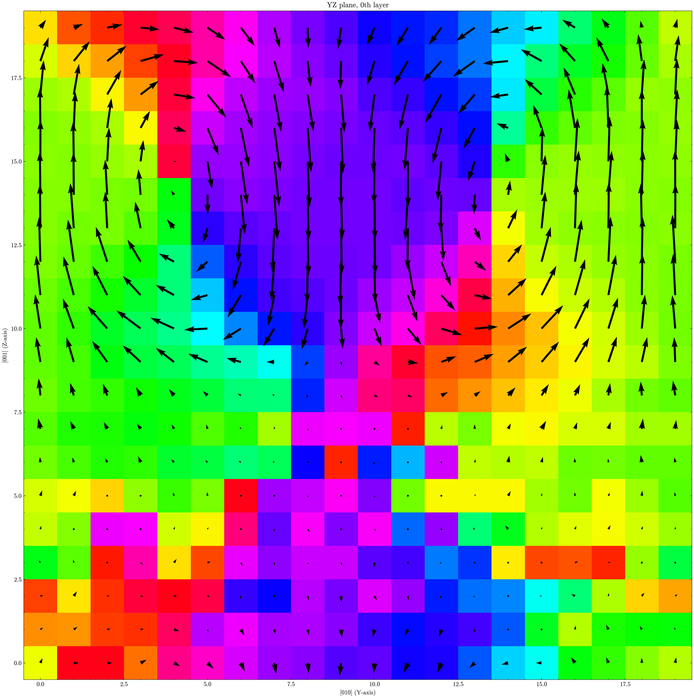
Step 4: plot displacement and polarization maps in real space
for f in *K.xyz; do
  tag="${f%.xyz}"
  gpumdkit.sh -plt plane-grid -i "${tag}-avg.xyz" -d "${tag}-disp.dat" -e Ti --select-xz 1 -o "plot-${tag}-disp"
  gpumdkit.sh -plt plane-grid -i "${tag}-avg.xyz" -d "${tag}-pol.dat" -e Ti --select-xz 1 -o "plot-${tag}-pol"
done
Step 5: build a temperature-order-parameter curve
By analyzing the lattice of each temperature-averaged structure together with its polarization (XX-pol.dat), we can obtain the following figure:
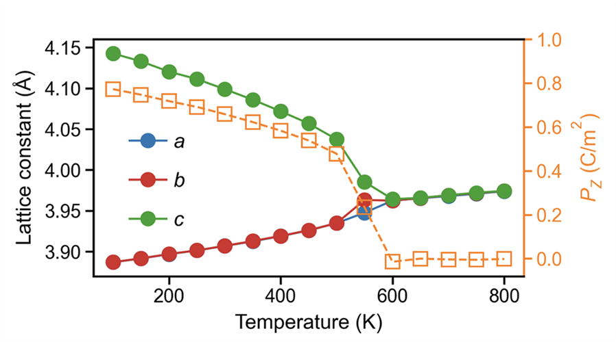
The trend shows a clear phase transition around 600 K, where the polarization vanishes.
Topological structure in PbTiO3/SrTiO3 superlattice
Assume movie.xyz is the trajectory of the PbTiO3/SrTiO3 superlattice in the current directory.
Step 1: build an averaged structure from the last 25% frames
Step 2: build the Ti neighbor list
Step 3: plot the plane-grid map
gpumdkit.sh -calc disp -i movie.xyz -n nl-Ti-O.dat -l 0.25 -o disp-last25.dat
gpumdkit.sh -plt plane-grid -i model-avg.xyz -d disp-last25.dat -e Ti --select-xy 0 -o plot-topology
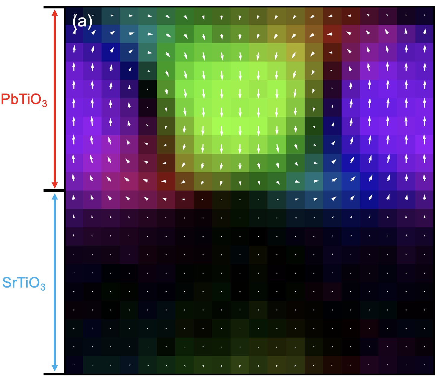
This gives a map similar to the one shown earlier. In the PTO region, a vortex-like polarization pattern is visible, while polarization in the STO region is close to zero.
Note: the example figure uses a custom colormap. The default GPUMDkit output uses a different style, which can be adjusted by editing the plotting script.
Other Systems
Organic-inorganic hybrid ferroelectrics
In many organic-inorganic ferroelectrics, polarization is strongly tied to anisotropic molecular units. A practical way to track molecular orientation is to use bond vectors.
For TMCM-CdCl3, you can use the C-Cl bond direction of the TMCM molecule as an orientation proxy, then use it to estimate the polarization state:
# Find the nearest Cl around each C (tune cutoff if needed)
gpumdkit.sh -calc nlist -i model.xyz -c 3 -n 1 -C C -E Cl -o nl-C-Cl.dat

# Compute C-Cl bond vectors from the trajectory
gpumdkit.sh -calc disp -i movie.xyz -n nl-C-Cl.dat -o ccl_vectors.dat
ccl_vectors.dat can then be analyzed as an orientation order parameter. More details could be found at: Phys. Rev. Lett. 136, 016801
Other ferroelectric families
Beyond ABO3, ferrodispcalc can be adapted to many ferroelectric systems, including nitrides, hafnia-based compounds, organic-inorganic hybrids, and some 2D ferroelectrics.