📊 Plot Scripts
The plotting module contains Python scripts for visualizing data generated by GPUMD, NEP, and GPUMDkit calculators. All plots can be displayed interactively or saved as high-resolution PNG files.
Script Location: Scripts/plt_scripts/
Quick Access
gpumdkit.sh -plt              # Show all plotting options
gpumdkit.sh -plt <type>       # Generate a plot
gpumdkit.sh -plt <type> save  # Save plot as PNG
gpumdkit.sh -plt <type> -h    # Show help for a specific plot type
Running gpumdkit.sh -plt prints the plotting command menu:
+-----------------------------------------------------------------------------------------------+
|                     GPUMDkit <version> PLOT & VISUALIZATION TOOLS              |
+-----------------------------------------------------------------------------------------------+
|  Usage: gpumdkit.sh -plt <type>                        Help: gpumdkit.sh -plt <type> -h       |
+-----------------------------------------------------------------------------------------------+
|                                    NEP Training & Evaluation                                  |
+-----------------------------------------------------------------------------------------------+
|  train          - NEP training results           prediction     - NEP prediction results      |
|  train_test     - NEP train and test results     parity_density - Parity density plot         |
|  train_density  - Training results density plot  restart        - Parameters in nep.restart   |
|  charge         - Charge distribution            born_charge    - Born effective charges      |
|  dimer          - Dimer energy/force curve       force_errors   - Force errors                |
|  des            - Descriptors                    lr             - Learning rate for gnep      |
+-----------------------------------------------------------------------------------------------+
|                                     Diffusion & Transport                                     |
+-----------------------------------------------------------------------------------------------+
|  msd            - Mean square displacement       msd_conv       - MSD convergence             |
|  msd_all        - MSD for all species            sdc            - Self diffusion coefficient  |
|  msd_sdc        - MSD and SDC together           sigma          - Arrhenius ionic conductivity|
|  D              - Arrhenius diffusivity          sigma_xyz      - Directional Arrhenius sigma |
|  D_xyz          - Directional Arrhenius D                                                     |
|  doas           - Density of atomistic states                                                 |
+-----------------------------------------------------------------------------------------------+
|                                    MD & Structural Analysis                                   |
+-----------------------------------------------------------------------------------------------+
|  thermo         - thermo info in thermo.out      thermo2/3      - Thermo in different styles  |
|  rdf            - Radial distribution function   rdf_pmf        - Potential of mean force     |
|  vac            - Velocity autocorrelation       cohesive       - Cohesive energy curve       |
|  net_force      - Net force distribution         plane-grid     - Displacement plane grid     |
+-----------------------------------------------------------------------------------------------+
|                                        Heat Transport                                         |
+-----------------------------------------------------------------------------------------------+
|  emd            - EMD results                    nemd           - NEMD results                |
|  hnemd          - HNEMD results                  viscosity      - Viscosity                   |
+-----------------------------------------------------------------------------------------------+
|                                          Phonons                                              |
+-----------------------------------------------------------------------------------------------+
|  pdos           - VAC and PDOS                                                                |
+-----------------------------------------------------------------------------------------------+
NEP Training and Prediction
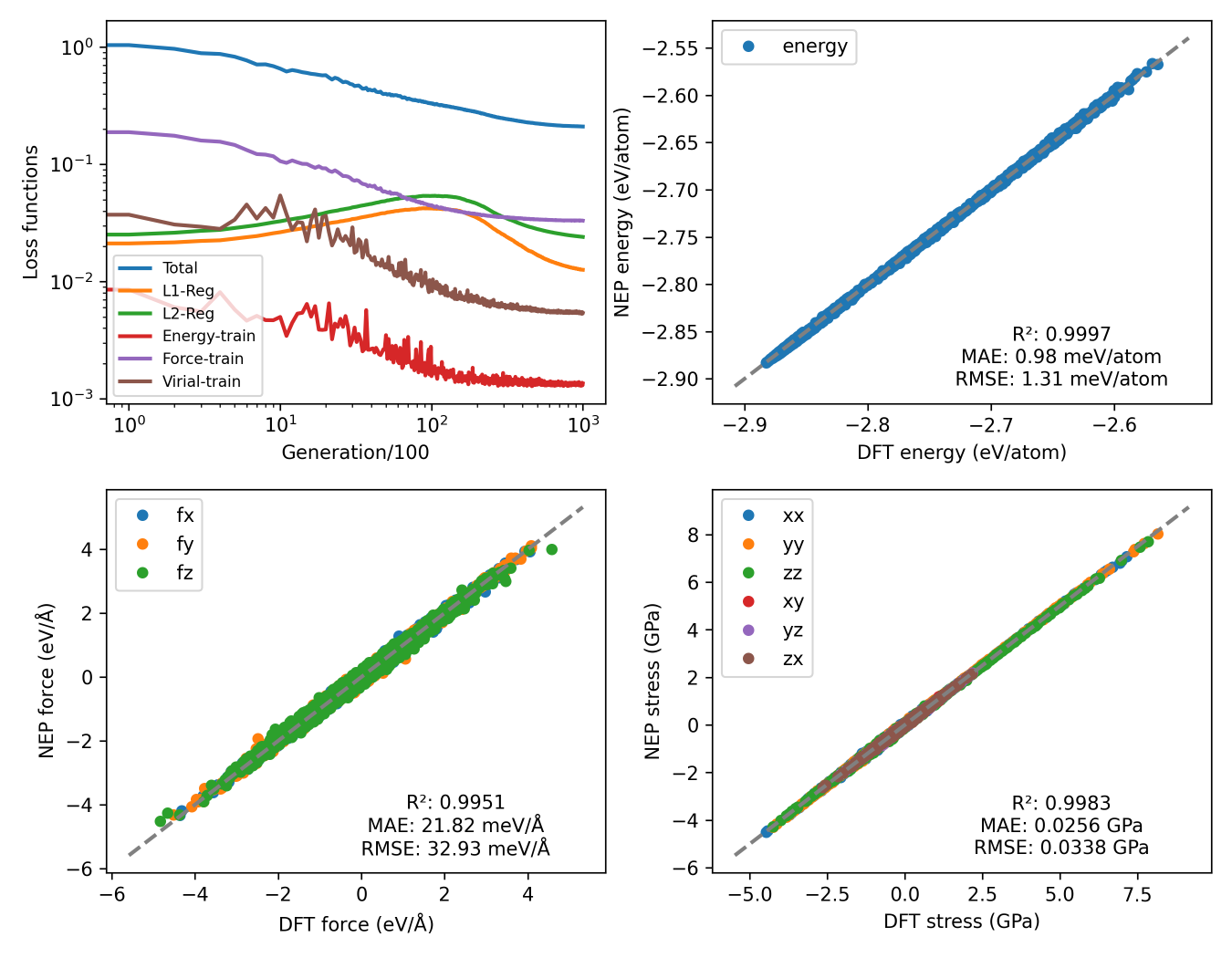
plt_train.py
Visualizes NEP training progress including loss curves, RMSE evolution, and parity plots comparing DFT vs NEP predictions for energy, forces, and stresses.
Input Files: loss.out, energy_train.out, force_train.out, virial_train.out
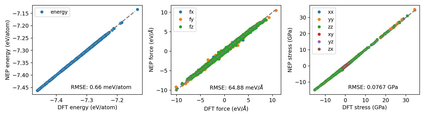
plt_prediction.py
Visualizes NEP prediction results on the test set.
Input Files: energy_test.out, force_test.out, virial_test.out
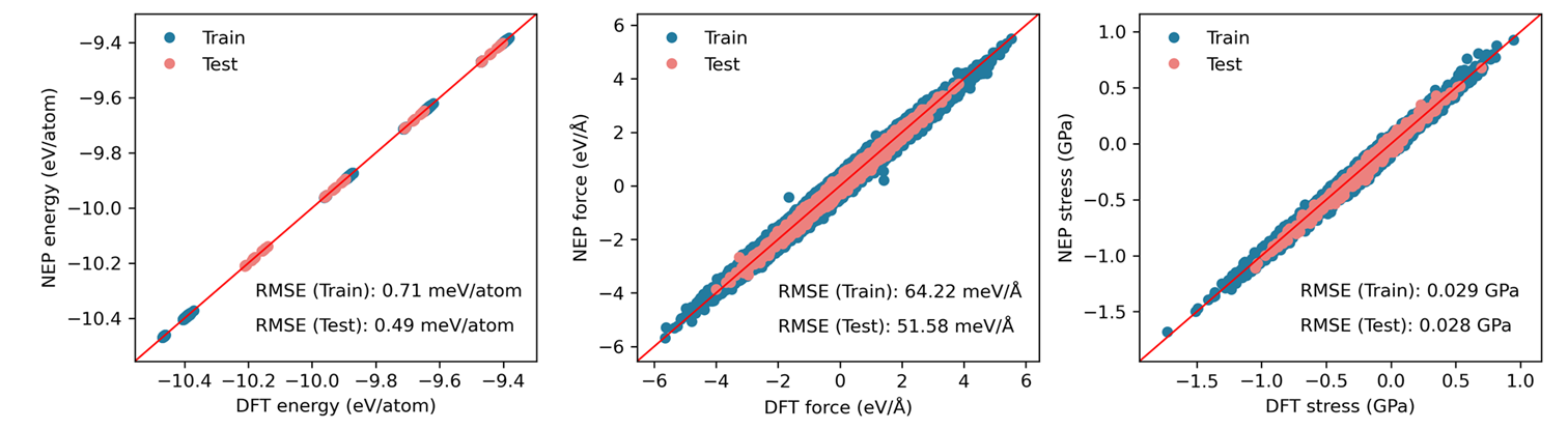
plt_train_test.py
Creates combined parity plots for both training and testing datasets.
Input Files: energy_train.out, force_train.out, virial_train.out, energy_test.out, force_test.out, virial_test.out
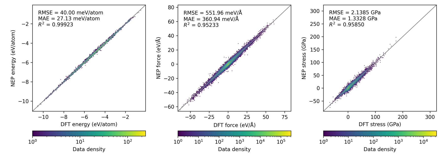
plt_parity_density.py
Generates density-based parity plots for energies, forces, and stresses. Useful for large datasets where scatter plots become unreadable.
Input Files: energy_train.out, force_train.out, virial_train.out
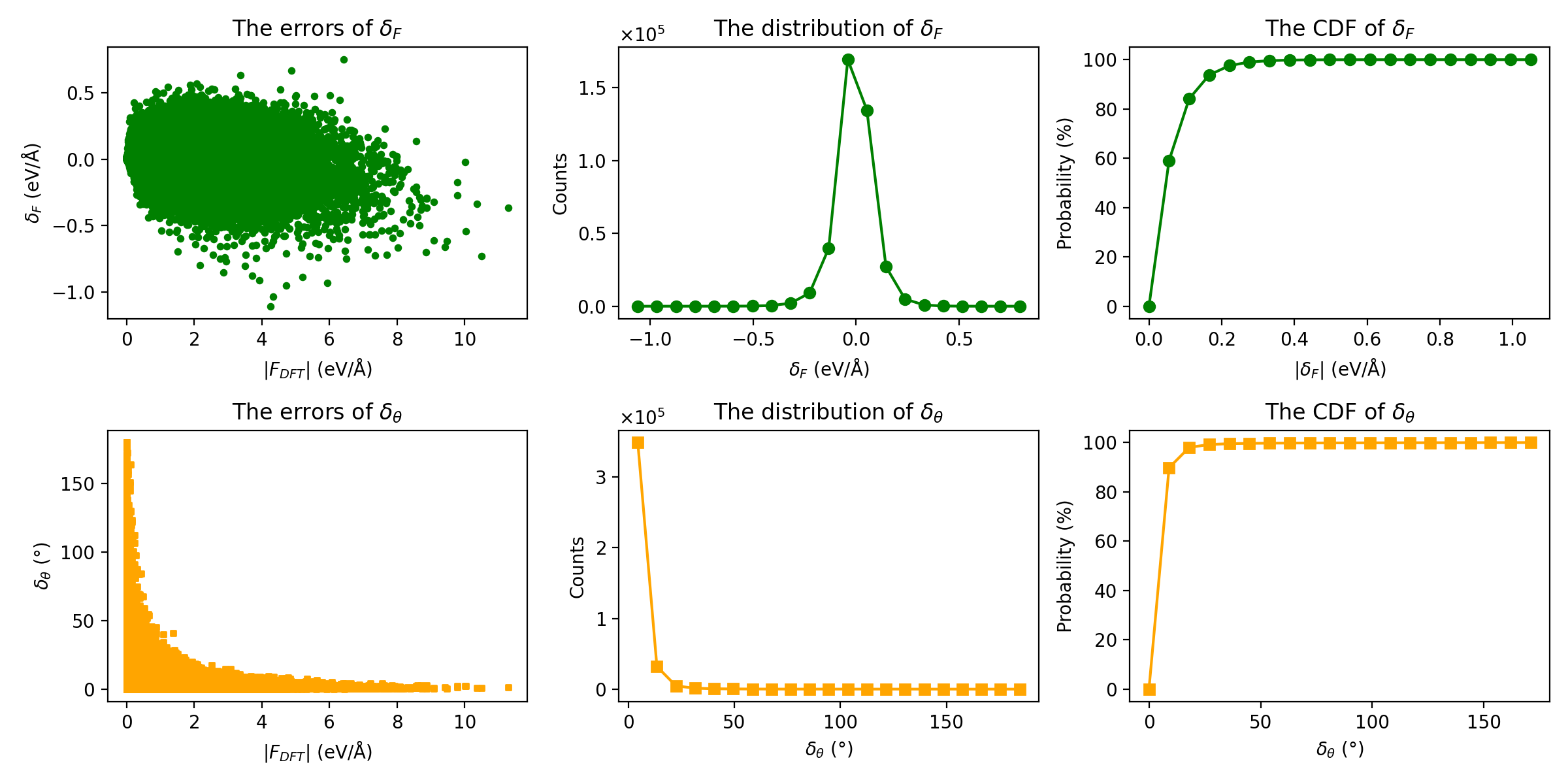
plt_force_errors.py
Plots force error evaluation metrics as proposed by Liu et al..
Input File: force_train.out
Metrics Displayed: - Force magnitude errors (delta_F) - Force angle errors (delta_theta) - Distribution of errors
plt_learning_rate.py
Visualizes learning rate during gnep training.
Input File: loss.out
Note: Only for the gnep training process.
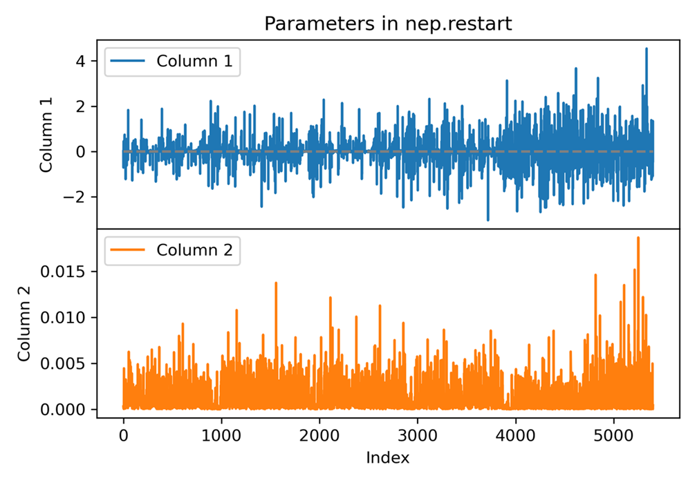
plt_nep_restart.py
Visualizes parameters stored in the nep.restart file.
Input File: nep.restart
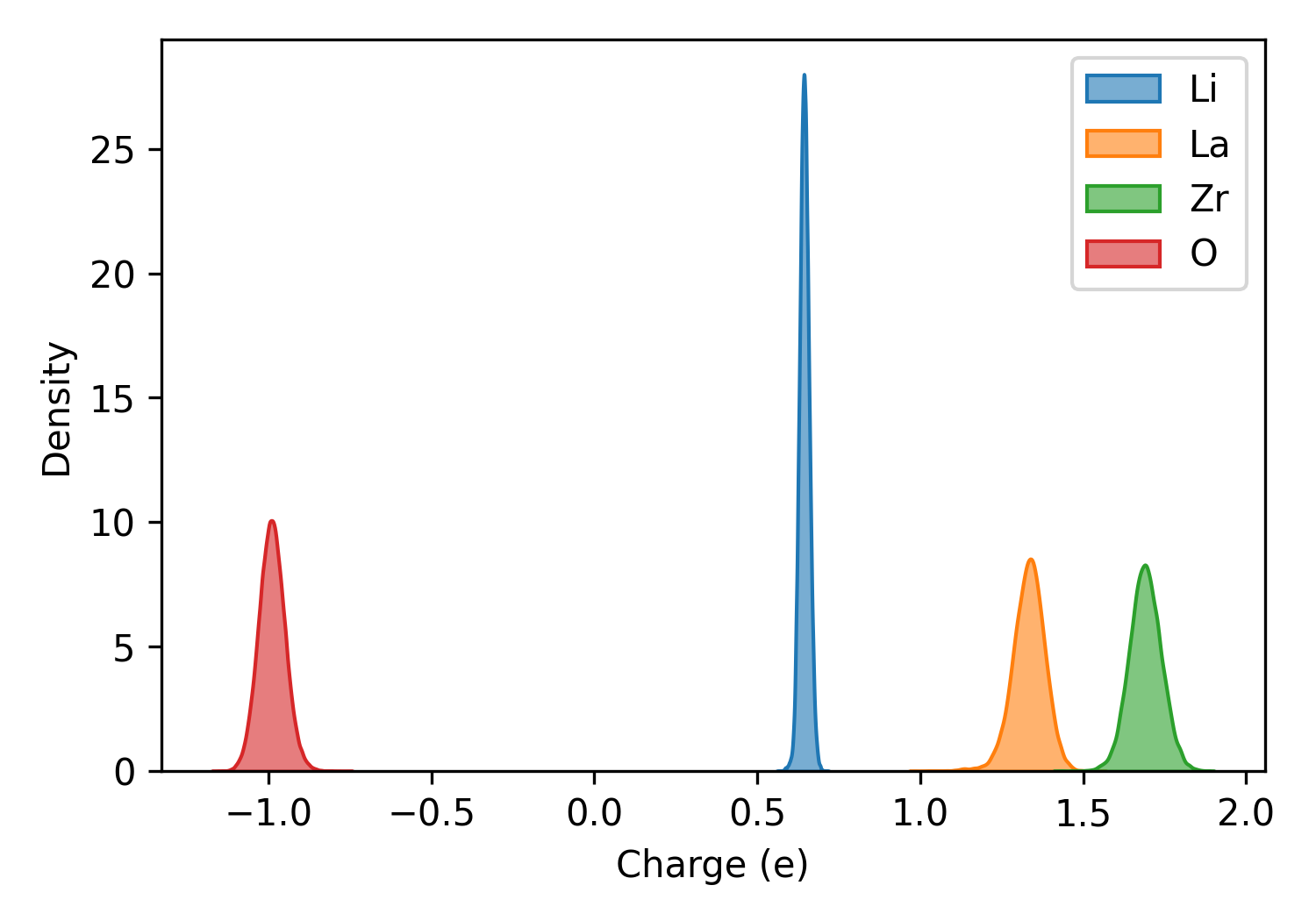
plt_charge.py
Plots charge distribution from qNEP model.
Input File: charge_train.out
Important: Ensure consistency between training set and charge output atom ordering. Use full batch training or run prediction step first.
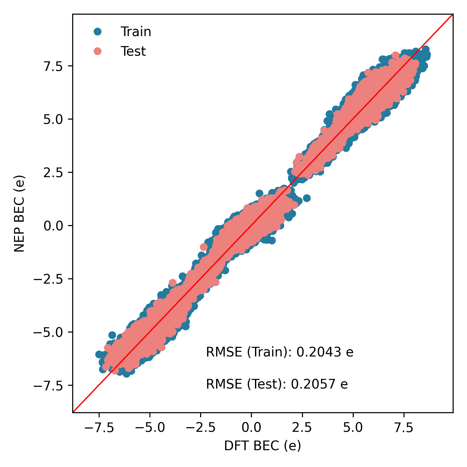
plt_born_charge.py
Creates parity plots for Born effective charges (BEC) on training and testing datasets. Structures with all-zero reference BEC are filtered out.
Input Files: bec_train.out, bec_test.out
Thermodynamic Properties
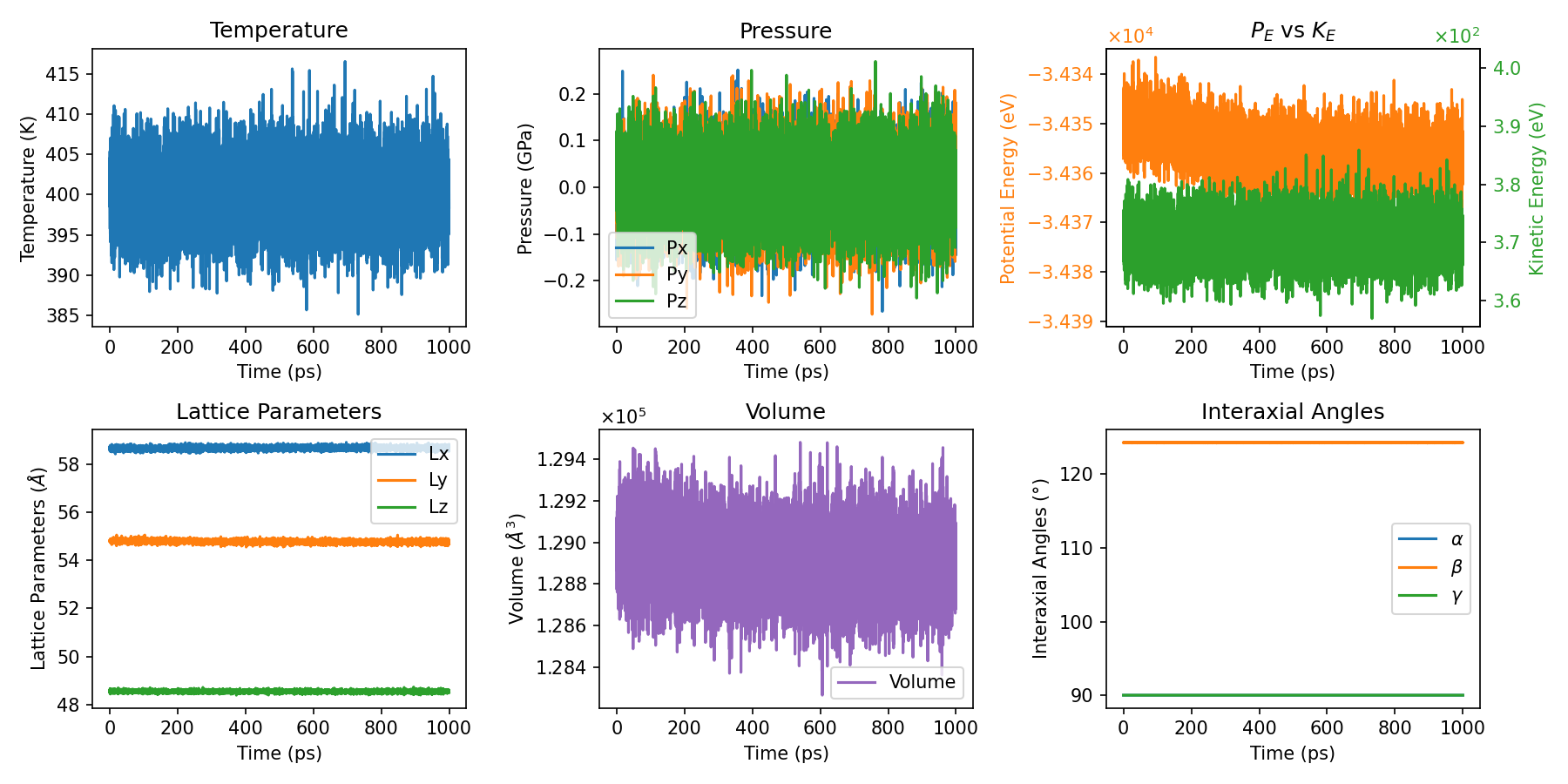
plt_thermo.py
Primary script for comprehensive thermodynamic property visualization.
Input File: thermo.out
plt_thermo2.py & plt_thermo3.py
Alternative thermodynamic visualization with different styles.
Input File: thermo.out
Diffusion and Ionic Transport
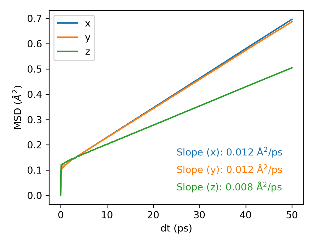
plt_msd.py
Plots mean square displacement (MSD) for all directions.
Input File: msd.out
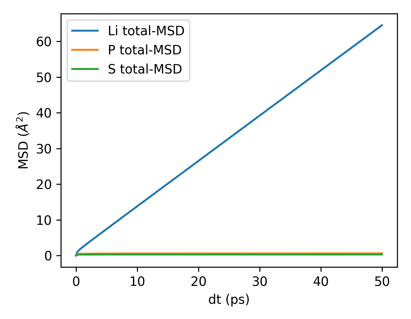
plt_msd_all.py
Plots MSD for all atomic species separately when using all_groups in GPUMD.
Input File: msd.out (computed with all_groups option)
Requirements: Must use all_groups in the compute_msd command in run.in.
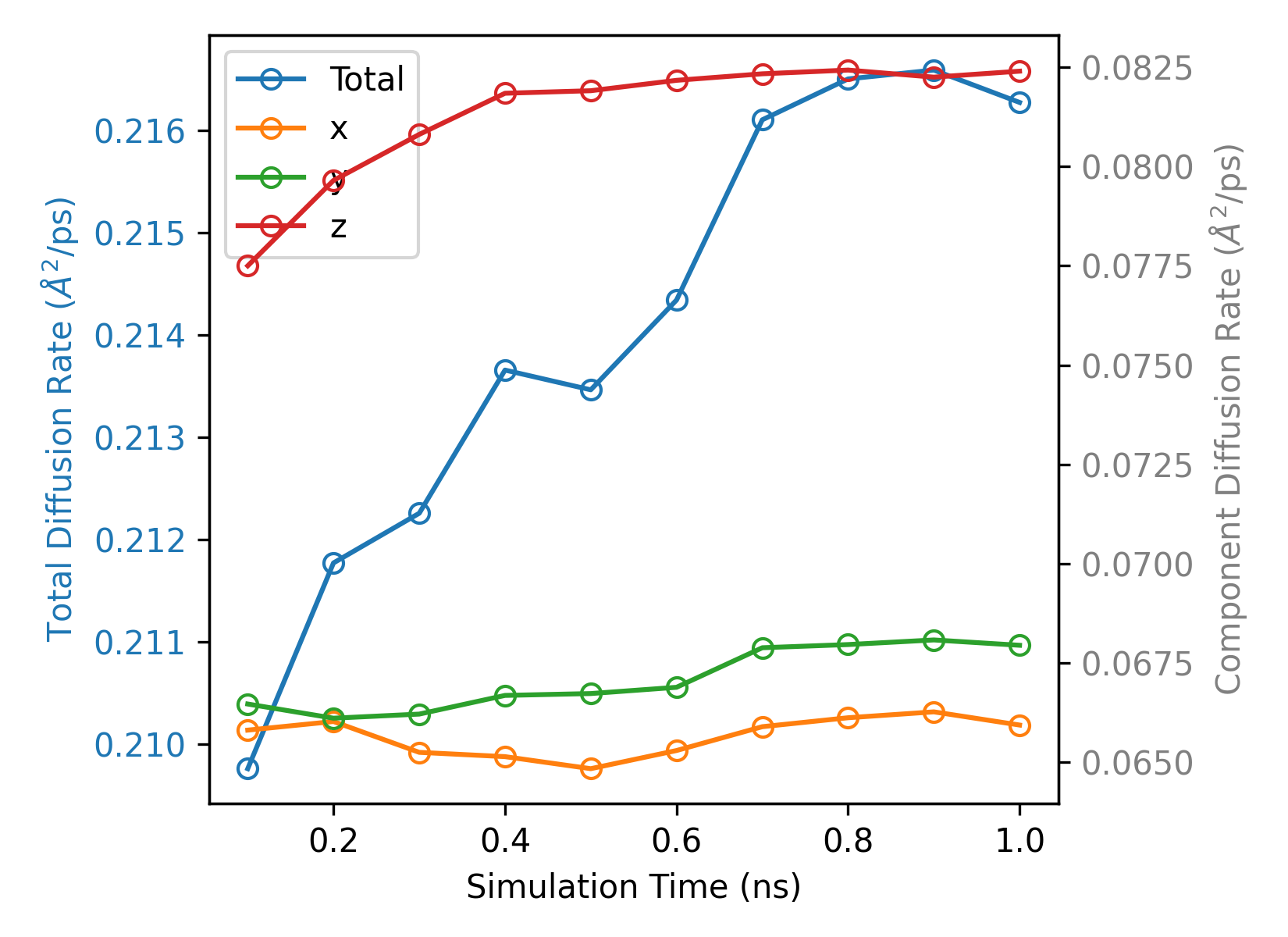
plt_msd_convergence_check.py
Checks convergence of MSD calculations across different time windows.
Input File: msd_step*.out (computed with save_every option)
Requirements: Use save_every in the compute_msd command.
Purpose: Verify MSD has converged sufficiently for accurate diffusion coefficient calculation.
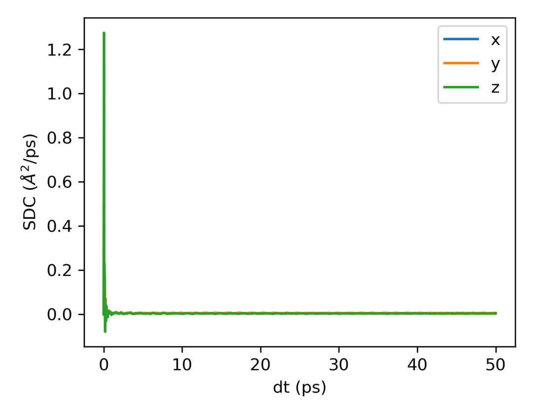
plt_sdc.py
Plots self-diffusion coefficient (SDC) vs time.
Input File: msd.out
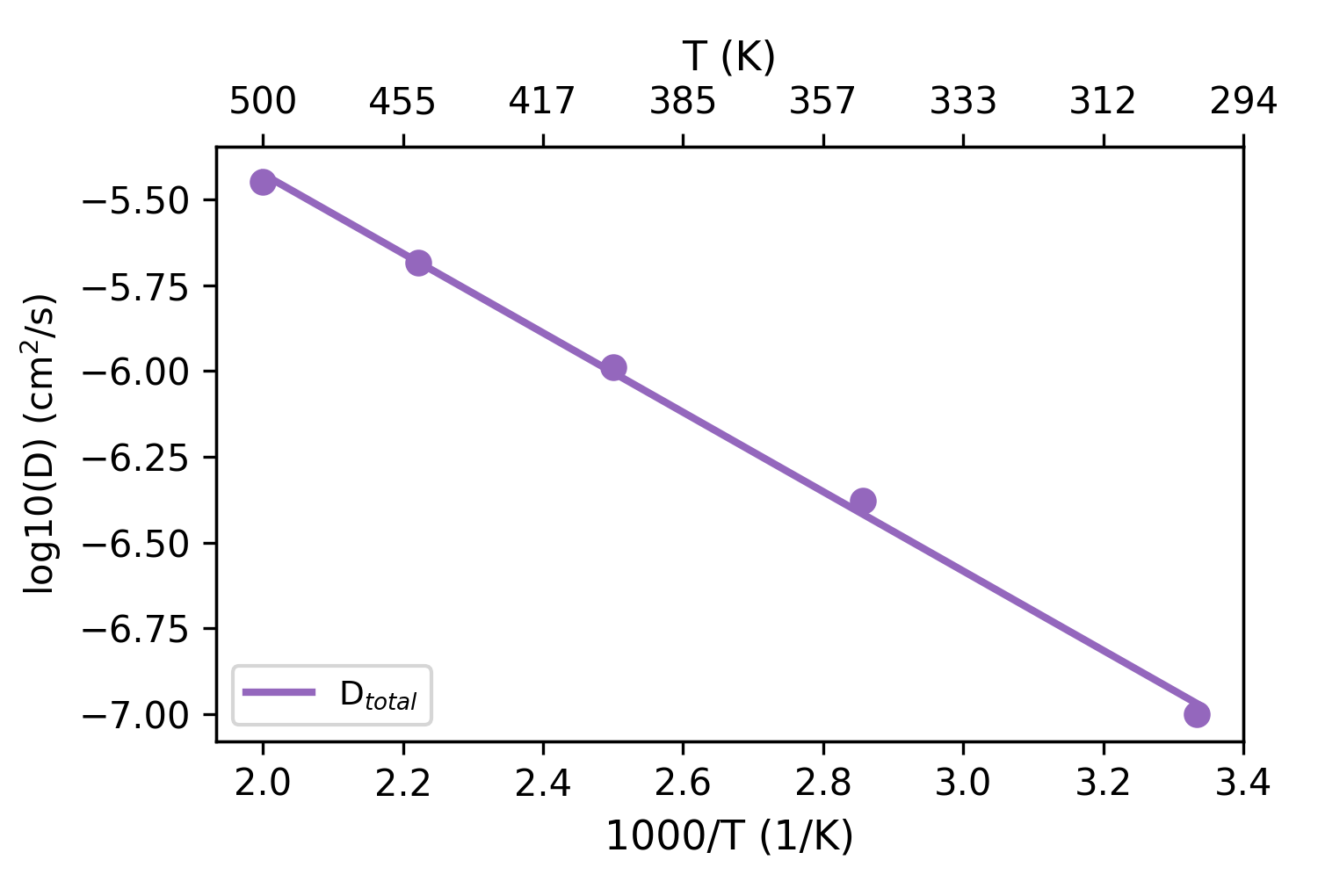
plt_arrhenius_d.py
Creates Arrhenius plot for diffusivity (log10 D vs 1000/T).
Input Files: *K/msd.out files (each temperature subdirectory should contain an msd.out)
Output example:
T: 300K, D_total: 1.001e-07 cm2/s
T: 350K, D_total: 4.184e-07 cm2/s
T: 400K, D_total: 1.027e-06 cm2/s
Ea: 0.230 eV
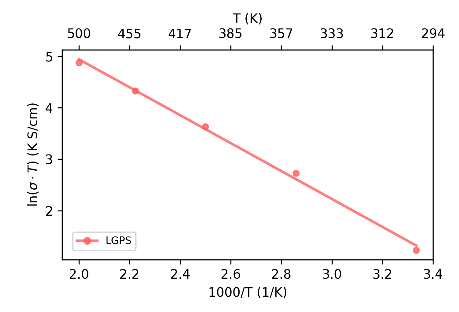
plt_arrhenius_sigma.py
Creates Arrhenius plot for ionic conductivity (ln(σ·T) vs 1000/T).
Input Files: *K/{model.xyz, run.in, thermo.out, msd.out} (each temperature subdirectory)
Heat Transport
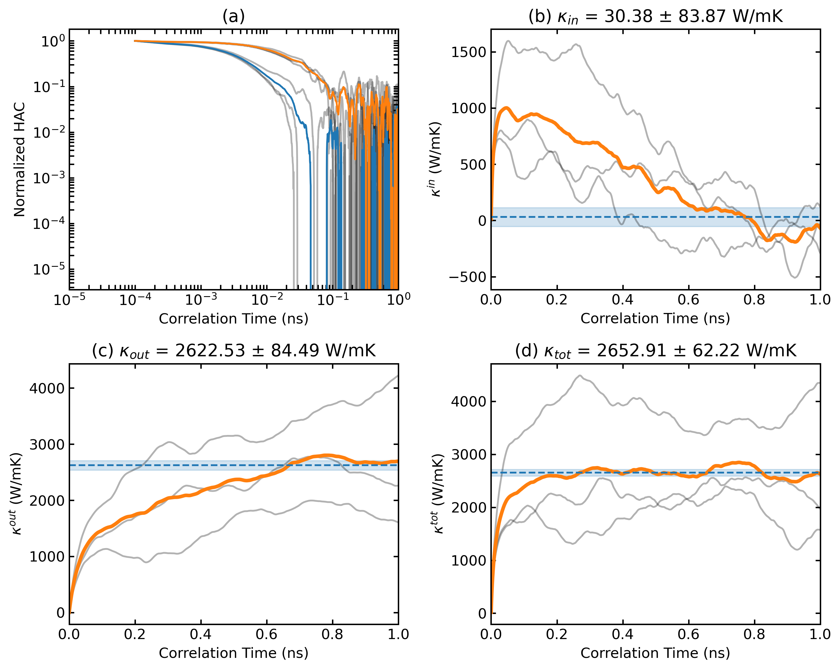
plt_emd.py
Analyzes and plots thermal conductivity from equilibrium molecular dynamics (EMD).
Input Files: EMD output files from GPUMD
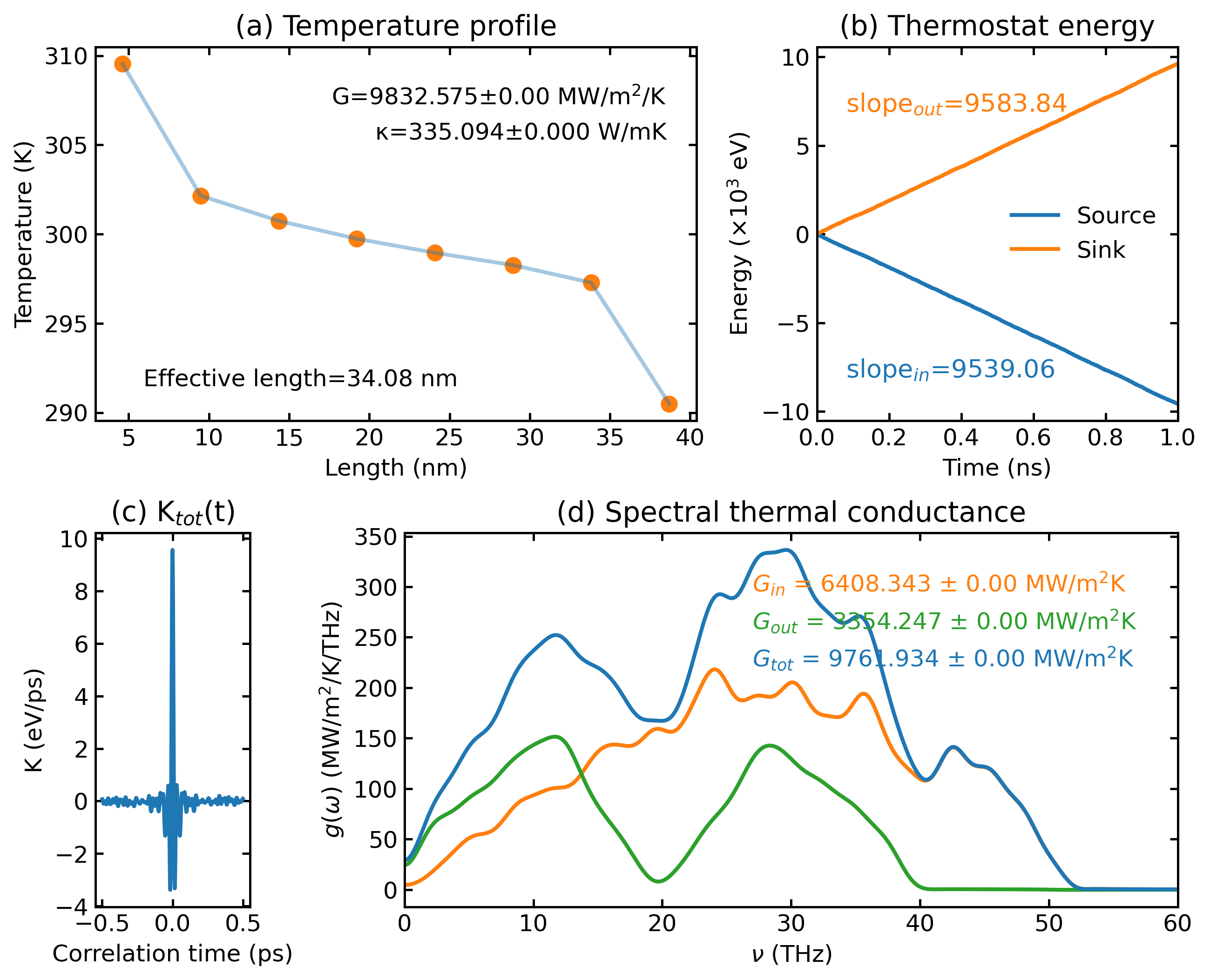
plt_nemd.py
Visualizes non-equilibrium molecular dynamics (NEMD) thermal transport properties.
Input Files: NEMD output files from GPUMD
Parameters:
| Parameter | Description |
|---|---|
real_length |
Real length of heat transfer zone in nm (set to Auto for auto-calculation) |
scale_eff_size |
Scale factor for effective cross-sectional area (default: 1). For 3D bulk: use 1. For low-dimensional systems with vacuum: S_box / S_eff |
cutoff_freq |
Cutoff frequency for SHC calculation in THz (default: 60) |
save |
Optional, save the plot as nemd.png |
Note: If no SHC data, set scale_eff_size and cutoff_freq to any number as placeholders when using save.
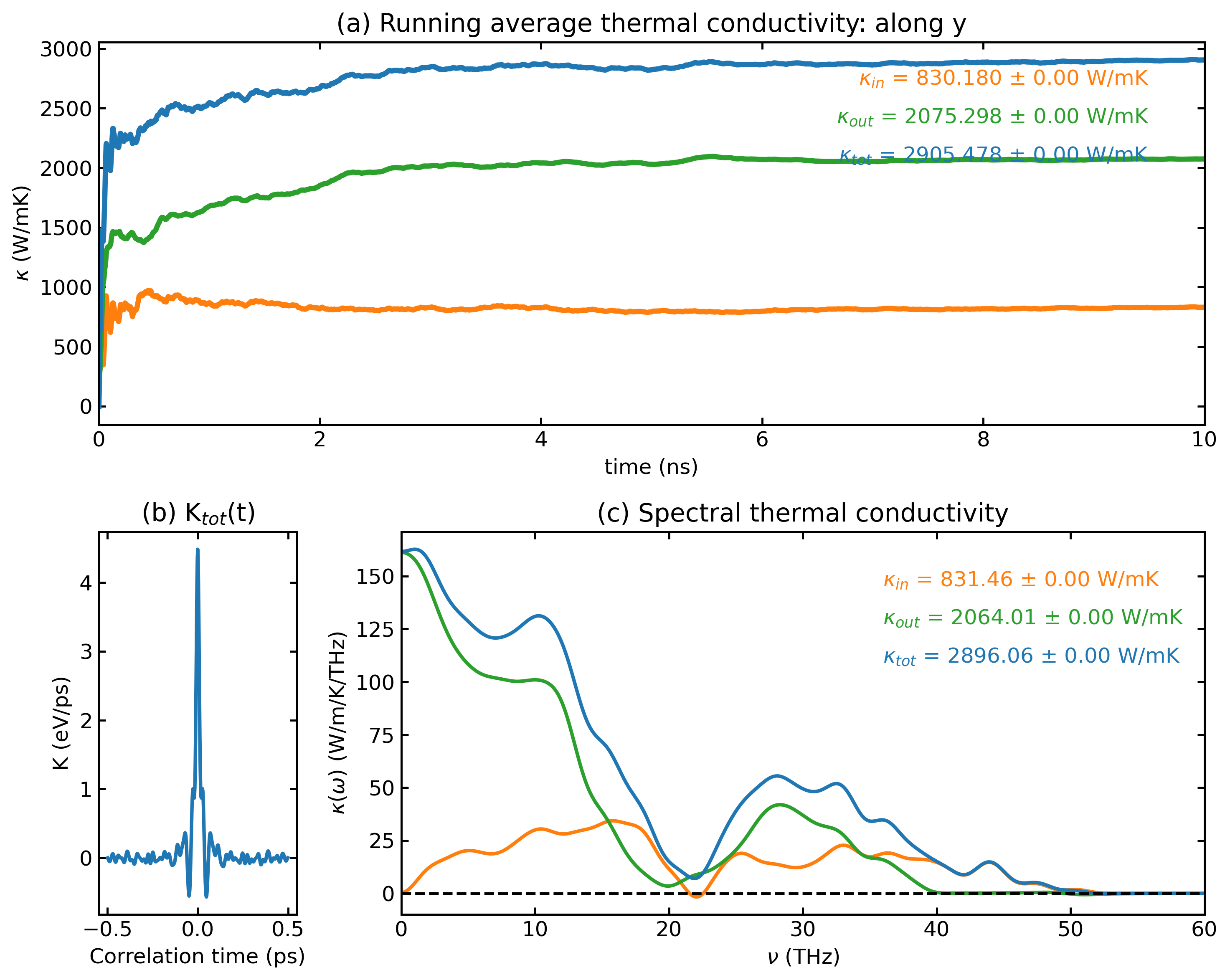
plt_hnemd.py
Plots homogeneous non-equilibrium molecular dynamics (HNEMD) results.
Input Files: HNEMD output files from GPUMD
Parameters:
| Parameter | Description |
|---|---|
scale_eff_size |
Scale factor for effective cross-sectional area (default: 1) |
cutoff_freq |
Cutoff frequency for SHC calculation in THz (default: 60) |
save |
Optional, save the plot as hnemd.png |
Note: If no SHC data, set scale_eff_size and cutoff_freq to any number as placeholders when using save.
Structural Analysis
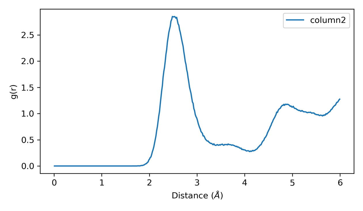
plt_rdf.py
Plots radial distribution function (RDF) showing pair correlations.
Input File: rdf.out
Full RDF output:
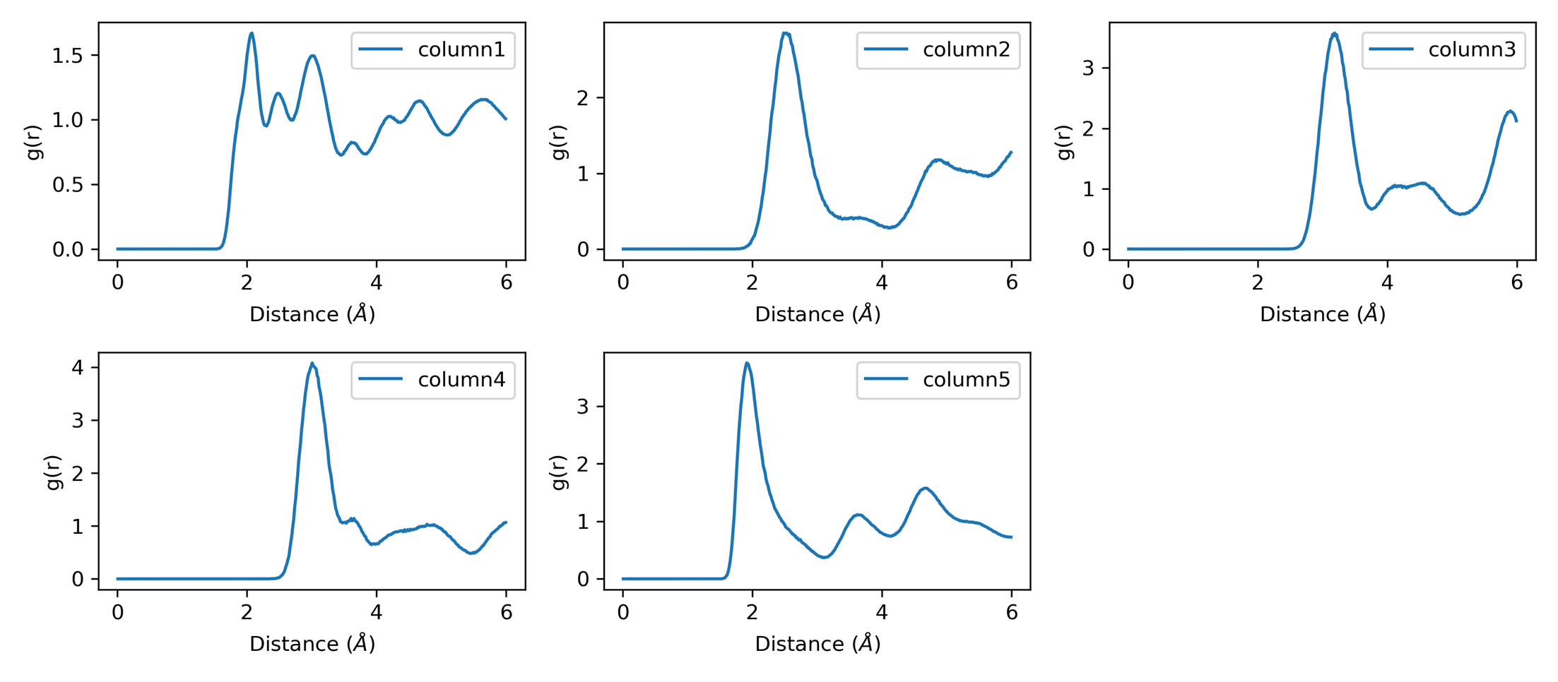
Single pair RDF:
plt_rdf_pmf.py
Plots RDF combined with potential of mean force (PMF).
Input File: rdf.out
plt_vac.py
Plots velocity autocorrelation function (VAC). Useful for analyzing phonon properties and atomic dynamics.
Input File: sdc.out (the VAC columns are read from this file by the plotting script)
Output: Interactive plot or vac.png (with save option)
plt_cohesive.py
Plots cohesive energy curve from cohesive.out. Useful for analyzing lattice stability and equilibrium lattice constants.
Input File: cohesive.out (isotropic scaling factor vs cohesive energy)
Output: Interactive plot or cohesive.png (with save option)
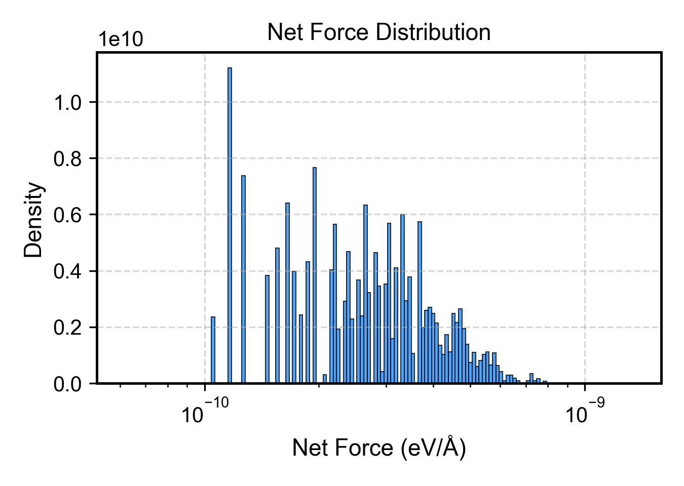
plt_net_force.py
Plots distribution of net forces on structures, useful for identifying problematic configurations.
Input File: train.xyz (extxyz format)
Reference: arXiv:2510.19774
Phonons
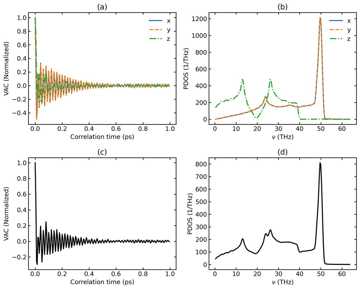
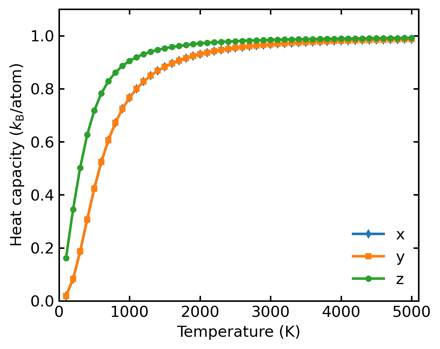
plt_pdos.py
Calculates and plots normalized VAC, PDOS, and Heat Capacity (Cv).
Input Files: model.xyz, run.in, dos.out, mvac.out
Heat capacity output:
Descriptor, Dimer, and Extra Analysis
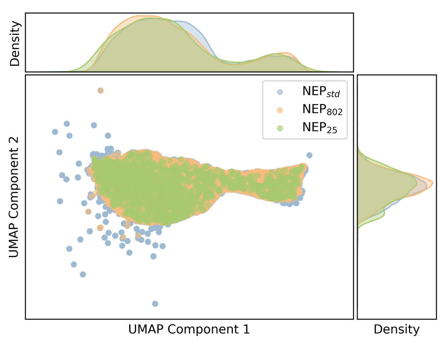
plt_descriptors.py
Visualizes high-dimensional NEP descriptors using dimensionality reduction (PCA or UMAP).
Input File: descriptors.npy (generated by gpumdkit.sh -calc des)
Methods:
- pca — Principal Component Analysis
- umap — Uniform Manifold Approximation and Projection
# First generate descriptors
gpumdkit.sh -calc des train.xyz descriptors.npy nep.txt Li

# Then visualize
gpumdkit.sh -plt des pca
gpumdkit.sh -plt des umap
plt_dimer.py
Plots dimer interaction curves. Two atoms are placed in a cubic box (30 Å) and the potential energy and force are calculated as a function of dimer distance using a NEP model.
Input File: nep.txt
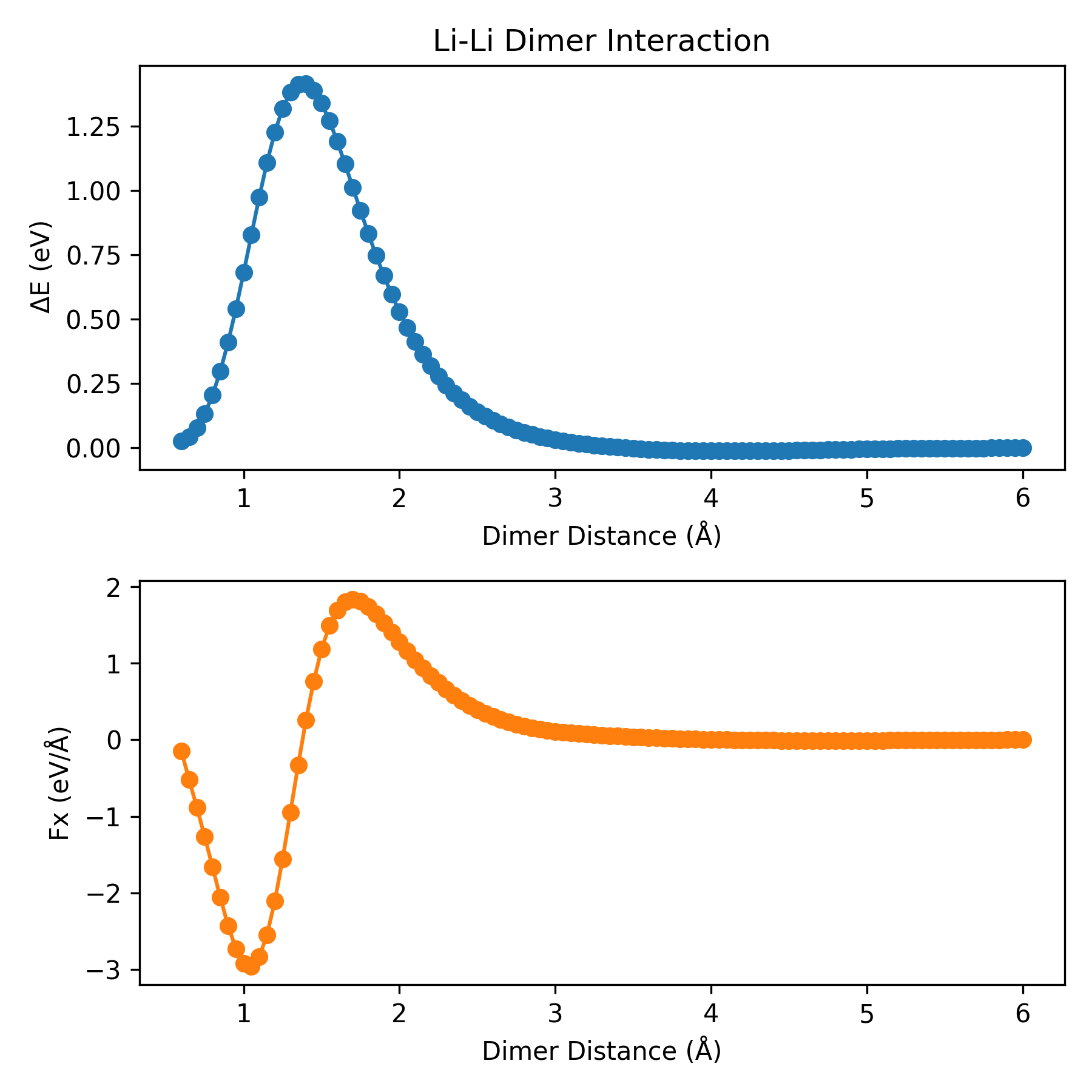
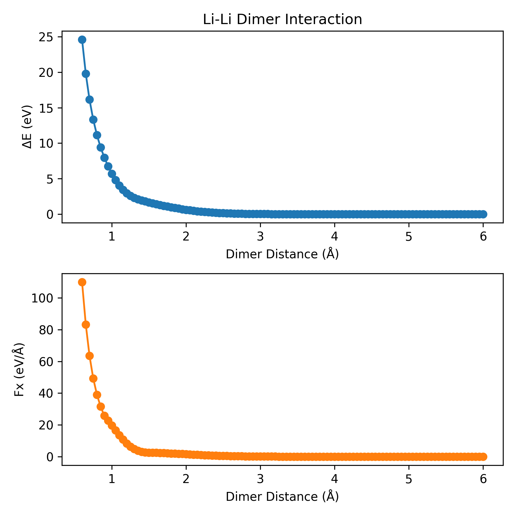
Reference: J. Chem. Inf. Model. 2026, 66, 3, 1406-1413
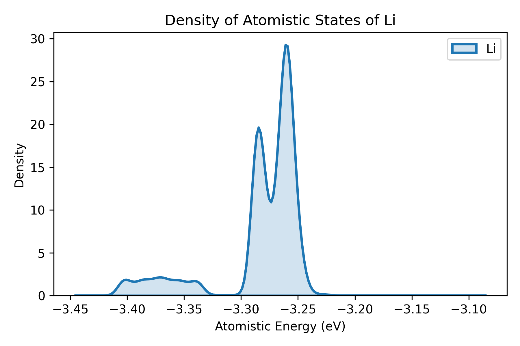
plt_doas.py
Plots density of atomistic states (DOAS) proposed by Wang et al..
Input File: doas.out (calculated by gpumdkit.sh -calc doas)
Plane-Grid Plot for Polar Materials
This workflow maps displacement or polarization data onto a grid and plots selected plane profiles. For detailed usage and real-world examples, see Polar Material Analysis.
Dependency:
Typical upstream steps:
gpumdkit.sh -calc nlist -i model.xyz -c 4 -n 12 -C Pb Sr -E O
gpumdkit.sh -calc disp -i movie.xyz -n nl-Pb_Sr-O.dat -o displacements.dat
gpumdkit.sh -calc avg-struct -i movie.xyz -l 0.2 -o averaged_structure.xyz
Usage:
gpumdkit.sh -plt plane-grid -i averaged_structure.xyz -d displacements.dat -e Pb Sr
gpumdkit.sh -plt plane-grid -i averaged_structure.xyz -d displacements.dat -e Pb Sr --select-xy 0 1
Quick Reference Table
| Command | Input File(s) | Description |
|---|---|---|
train |
loss.out, *_train.out |
NEP training plots |
prediction / test |
*_test.out |
NEP prediction plots |
train_test |
*_train.out, *_test.out |
Combined parity plots |
parity_density |
*_train.out |
Density-based parity plots |
force_errors |
force_train.out |
Force error metrics |
lr |
loss.out (gnep) |
Learning rate |
restart |
nep.restart |
Restart file parameters |
charge |
charge_train.out |
Charge distribution |
born_charge / bec |
bec_train.out, bec_test.out |
Born effective charges |
thermo |
thermo.out |
Thermodynamic properties |
msd |
msd.out |
Mean square displacement |
msd_all |
msd.out (all_groups) |
MSD for all species |
msd_conv |
msd_step*.out |
MSD convergence check |
sdc |
msd.out |
Self-diffusion coefficient |
arrhenius_d / D |
*K/msd.out |
Arrhenius diffusivity |
arrhenius_sigma / sigma |
*K/{model.xyz, run.in, thermo.out, msd.out} |
Arrhenius ionic conductivity |
rdf |
rdf.out |
Radial distribution function |
rdf_pmf |
rdf.out |
RDF + potential of mean force |
vac |
sdc.out |
Velocity autocorrelation |
cohesive |
cohesive.out |
Cohesive energy curve |
net_force |
train.xyz |
Net force distribution |
doas |
doas.out |
Density of atomistic states |
des |
descriptors.npy |
Descriptor PCA/UMAP |
dimer |
nep.txt |
Dimer energy/force curve |
pdos |
model.xyz, run.in, dos.out, mvac.out |
VAC and PDOS |
emd |
EMD outputs | EMD thermal conductivity |
nemd |
NEMD outputs | NEMD thermal transport |
hnemd |
HNEMD outputs | HNEMD thermal transport |
viscosity |
Viscosity outputs | Viscosity |